workshops
Introduction to QGIS
For anyone who is new to QGIS, you can find tutorials here and references from our previous workshop to help you getting started.
Raster processing on the command-line
A short introduction to raster processing using command line tools.
Installation
We’ll be passing around thumbdrives containing all the files we’ll need to interact with over the course of the presentation. Please copy those files onto an accessible location on your laptop.
Next, we’ll need to our a terminal from which to run our commands from. Once open, cd into the directory.
In order to ensure that we’ll be working with the environments we’re going to make use of Docker images. There should be a Docker installation script provided for Windows and OSX machines.
Once docker is installed, we can load the blr.tar file, which contains a Docker image containing all the dependencies which we’ll need.
# 1
docker load < blr.tar
Once you’ve download the Docker image, we can run it via:
# 2
docker run --volume $(pwd):/data -it 571f6261f338 /bin/bash
This will mount the local directory $(pwd) on your own machine, to the /data directory within the Docker container. In other words, any files you create in /data will also be accessible locally.
We’ll need to do one last thing in order to get access to the packages which we’ll be using.
# 3
source /tmp/venv/bin/activate
cd /data
Getting started
My favorite way to search around for Landsat imagery is via Vincent Sarago’s SatelliteSearch. The Landsat path & row which encompasses Bangalore is 144, 51, which is what we’ll be working with today.
Let’s see what imagery is available. We can use the landsat package here, to filter for the path and row, as well as the maximum amount of cloud coverage.
landsat search --pathrow 144,51 --cloud 10
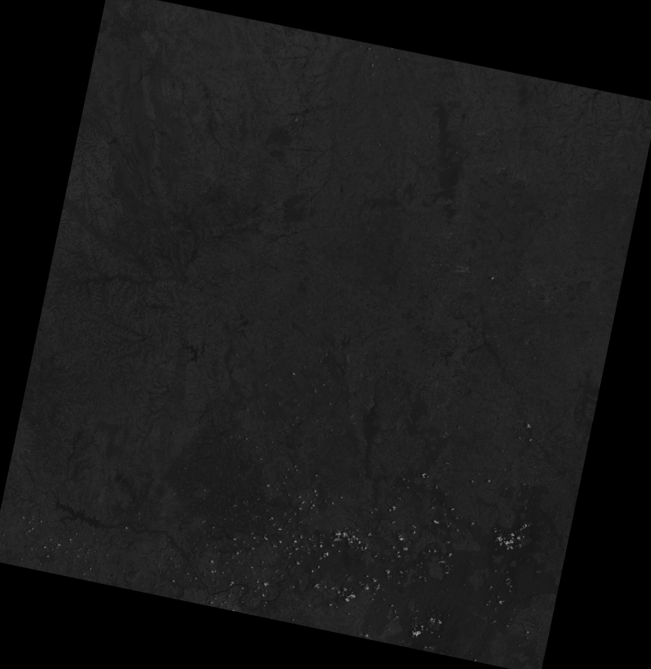
We’ve already downloaded the LC81440512016096LGN00 scene — let’s take a look at it’s metadata.
# 4
cd LC81440512016096LGN00/
ls -ll
Let’s take a look at some of the metadata for that image.
# 5
rio info --indent 4 /data/LC81440512016096LGN00/LC81440512016096LGN00_B4.TIF
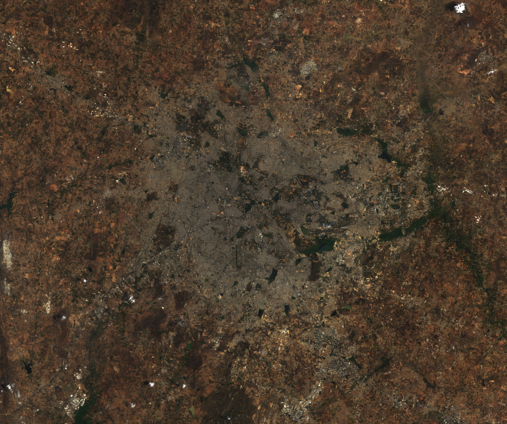
Next, we’re going to need to turn the individual images into a single RGB image.
# 6
landsat process /data/LC81440512016096LGN00 --bands 432
mv /root/landsat/processed/LC81440512016096LGN00/LC81440512016096LGN00_bands_432.TIF 432.TIF
Let’s take a look at metadata for our new image.
# 7
rio info --indent 4 432.TIF
What we have is great, but it’s a bit more information than we need. Let’s clip this imagery to the city of Bangalore. I like to use geojson.io to draw boundaries. You can easily export the bounds as a geojson, which is what we’ll use to clip our Landsat imagery with.
In your directory, you can find a clip-3857.geojson file, which describes the extents around Bangalore which we’ll chop.
# 8
rio clip 432.TIF 432-clipped.TIF --bounds=$(fio info clip-3857.geojson --bounds)
Not bad, but we could make this a little more beautiful using rio color
# 9
rio color 432-clipped.TIF bangalore.TIF sigmoidal RGB 5 0.5
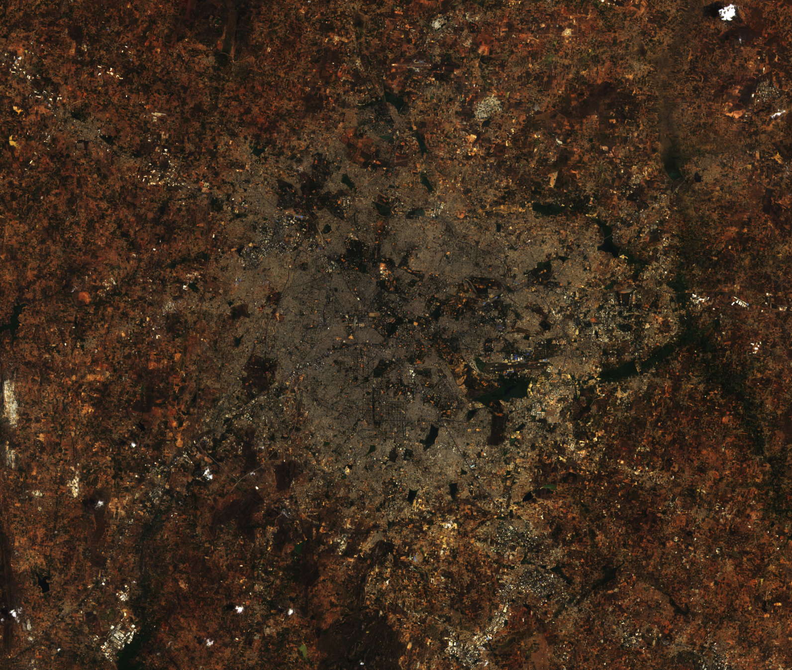
These edits are pretty tame, but feel free to go crazy! Check out the documentation for some ideas.